Graphing with Senior Physics
Video of line graphs with excel.
Below is a video outlining how I used Excel to construct line graphs with Senior Physics Classes.
Below are the original excel files that the above video and instructions below outline.
| refractive_index_of_perspex.xlsx |
| photoelectric_lab_results.xlsx |
Line graphs with excel - outline.

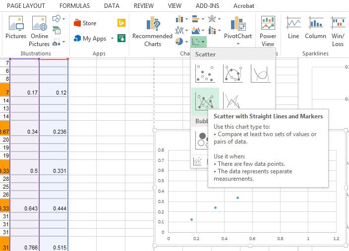
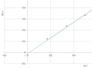
1. To create a line graph I first highlight the cells of the excel table I wanted graphed. In this case it was the sine of the angle of incidence (sin i) against the sine of the angle of refraction (sin r) as shown to the right.
2. Next I chose what type of graph was required and since both axes includes continuous data then a line graph was chosen. I used a scatter graph with lines as shown below.
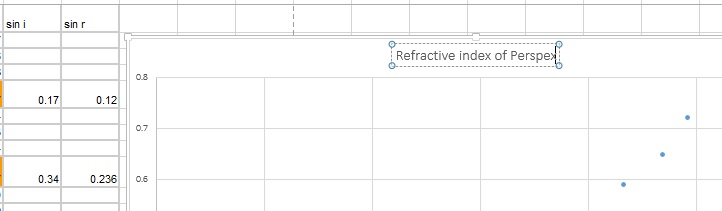
3. I then changed the title to a descriptive one as shown below by clicking in the box and typing.
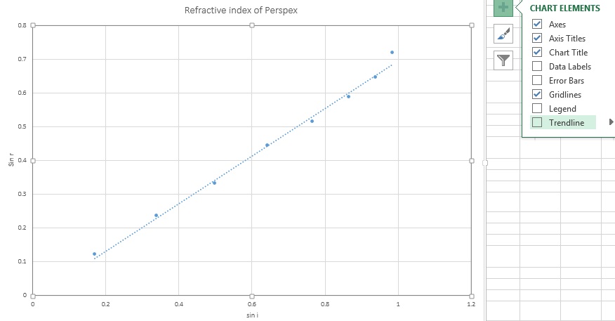
4. Axes labels were then needed so I clicked on the 'plus' sign that appears at the top right hand corner of the graph when the pointer is placed onto the graph and selected 'Axis Titles'.
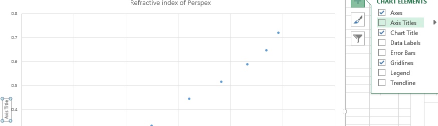
5. I then types 'sin r' and 'sin i' into the relevant axes and then selected 'Trendline', as shown below, to put a 'line of best fit' into the graph. Now it is starting to look like a real scientific graph.
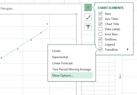
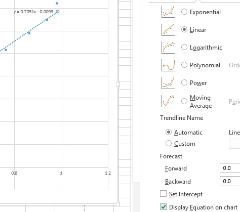
6. I needed the line to be extrapolated towards the origin of the graph, to do this I needed to select the arrow to the right of 'Trendline' and then select 'More Options...'
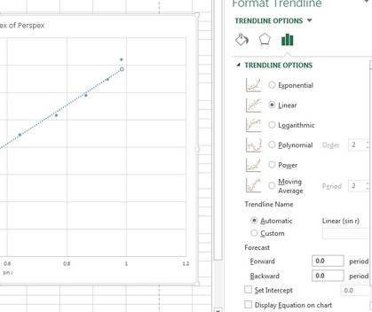
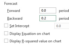
7. To extend the line back towards the origin I typed in the 'Backward' box '0.2'.
|
|
8. As can be seen in the image to the left the line extended to be very close to the origin with negative values now part of the graph. Being close to the origin means the systematic errors in the execution of the experimental method was very low meaning it was a very well done activity.
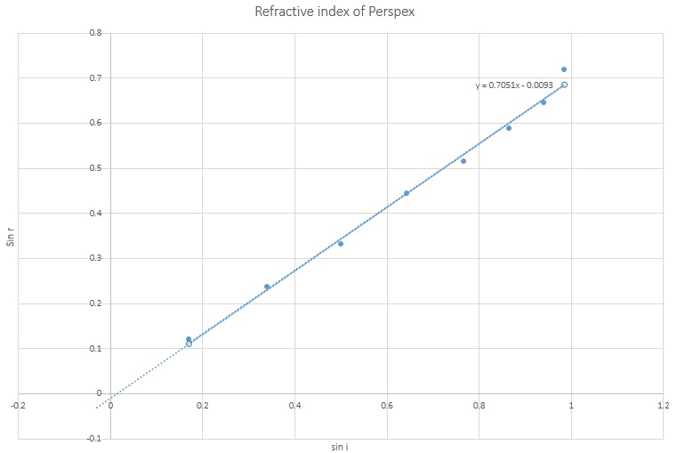
9. I then wanted the equation of the straight line to be displayed on the graph so the 'refractive index' of the perspex block could be determined from the graph. To do this I clicked on the plus symbol again, as earlier, and ticked the check box next to 'Display Equation on chart' as shown below.
10. Here is the final result including the equation of the line. Since y = mx + b then the gradient is 0.7051. Because the refractive index is, n = sin i/sin r then the inverse of the gradient needed to be found. Students then calculated the refractive index to be 1.42. The literature value is 1.495 .
11. Below is another graph used with a Senior Physics class as part of a computer simulation of the 'photoelectric effect' that was an assessment task. Students had to collect data and construct a graph as shown below.
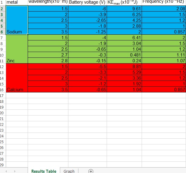
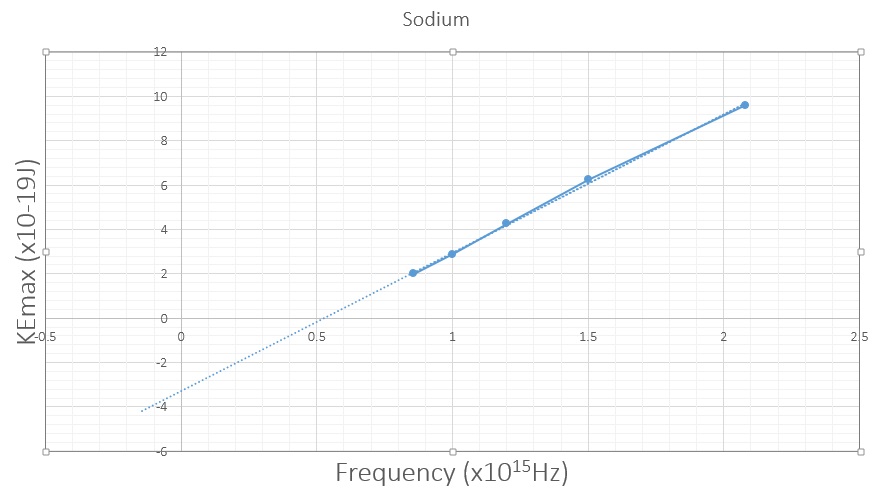
12. Line graphs then needed to be completed for each of the 3 metals analysed. Below is a graph for Sodium which was set up in the same manner as outlined previously.
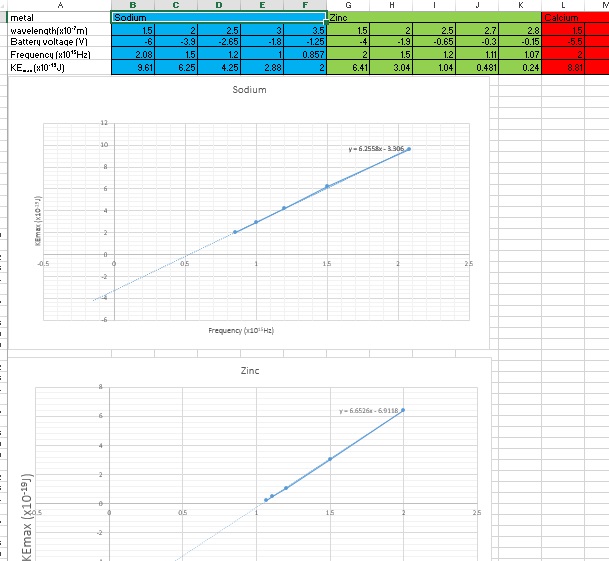
13. To do this the 'frequency' and 'Kinetic Energy' rows of the 'sodium' data were highlighted bringing up the graph below.
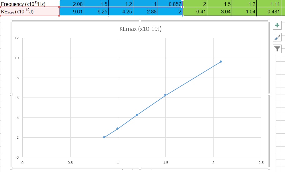
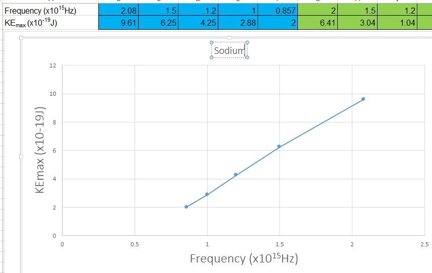
14. The axes and title were constructed as outlined earlier.
15. The trendline was then generated and extended to beyond the 'y-axis'
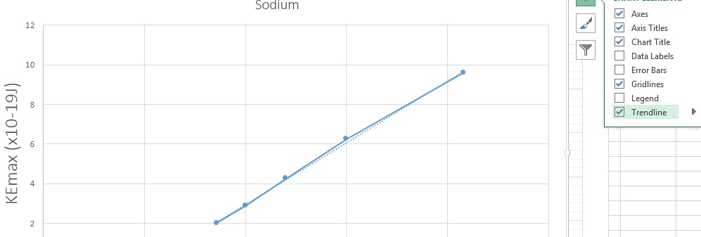
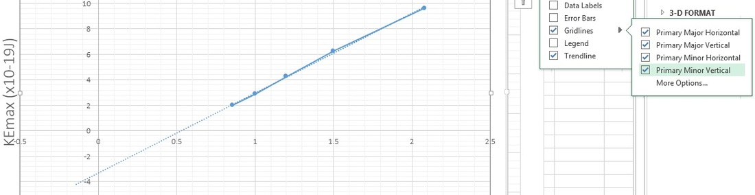
16. In this graph I also included minor grid lines, as I often prefer, by clicking on the arrow to the right of 'Gridlines' and selecting the last two check boxes as shown below.
Here is the final graph.