Year 10 Results.
Below is a video outlining my use of excel using a very large excel spreadsheet to analyse student results from two curricula. The video is 28 minutes long! But there is s lot to go through with this hefty spreadsheet. A summary of the video the use of excel is given on this page with screenshots below the video. A copy of the original spreadsheet for downloading is also provided below the video. This spreadsheet was adapted from one worked on by Jennie Young who was head teacher of Science at St Paul's Grammar School, Penrith when it was made.
Excel is a very powerful tool for teacher administration of data. The file below is a spreadsheet containing a lot of data from a year 10 cohort back in 2010 that were assessed from two different curriculum, the NSW Board of Studies and the International Baccalaureate Middle Years Program.
| year_10_spreadsheet_2010_anon.xlsx |
At My current school excel is not extensively used in my faculty for Administration purposes apart from my use as we use ‘edumate’ to enter marks and write reports. I, however, like excel for its flexibility and to generate detailed data on students. Because I have no access to a whole years worth of data for a whole year group at my current school I have used a spreadsheet from my previous school and modified it to demonstrate my excel skills and knowledge. This spreadsheet includes data for 125 year 10 students who were assessed in both the NSW Board of Studies (BOS) School Certificate as well as the International Baccalaureate (IB) Middle Years Program (MYP). This complicates assessment beyond that of many schools and as such Microsoft excel is a very useful tool in analysing such results in grading and reporting.
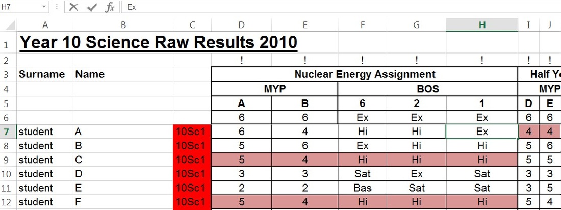
When a huge amount of data is required it is useful to create multiple ‘tabs’ in excel. The first one in this spreadsheet is called ‘Raw’ as it has the raw results throughout the year.
Even though this tab has raw marks formulae are still useful and can contribute to reducing workload in marking two credentials (BOS and MYP). For example, in marking the Nuclear energy assignment, the MYP criterion F was used: 'Attitudes in Science- Organization, team-working, manipulative and other lab skills' which is equivalent to BOS outcome ‘4’, so rather than marking the same thing twice to come out with an MYP grade out of 6 or a BOS ‘Course Performance Descriptor' (CPD) up to excellent, I used excel to convert the BOS grade to an MYP grade.
To do this an ‘IF’ statement formulae is written, for example:
=IF(L7="non",1or0,IF(L7="Min",2,IF(L7="Bas",3,IF(L7="Sat",4,IF(L7="Hi",5,IF(L7="Ex",6))))))
To add the marks up for the half yearly examination, the previous spreadsheet had a formula for column ‘R’: =N7+O7+P7+Q7, however I have learned that this is not the most efficient way to do it and have now changed the formula to: =sum(N7:Q7). This is especially useful when many columns or rows need adding.
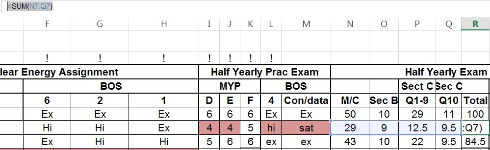
I put in another ‘IF’ statement into column ‘S’ as section C, Question 10, in the Half Yearly exam related to MYP criterion ‘C’ “Scientific Knowledge and Concepts”. Because MYP grades are 1 to 6 them the mark out of 11 needed to be converted into a maximum of 6:
=IF(Q7<=1,1,IF(Q7<=3,2,IF(Q7<=5,3,IF(Q7<=7,4,IF(Q7<=9,5,IF(Q7<=11,6))))))
This question also related to a BOS outcome ‘3’ in column U. the mark was just left out of 11.
No formulae were used for the ‘Ethics of Genetics’ task for MYP or BOS as this was marked via a rubric and the marks just manually entered from them.
For the yearly exam I wanted to rank the students. The program that my school used, as does my current school as well, ranks results automatically so excel is not needed for this in my context. However I have added in a ranking column to demonstrate this. I actually now do use this feature even though I do not have to as it is easy and effective to see students ranks before entered into the online school based software.
With ranking ‘$’ signs are needed as shown below. This is to keep the ranking of each row (student) based upon rows 7 to 131. If $ not used then row AD8 would be ranked based on AD8 to AD132 rather than AD7 to AD131 as all students should be ranked from.
=RANK(AD7,AD$7:AD$131)

|
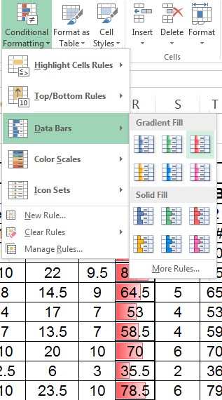
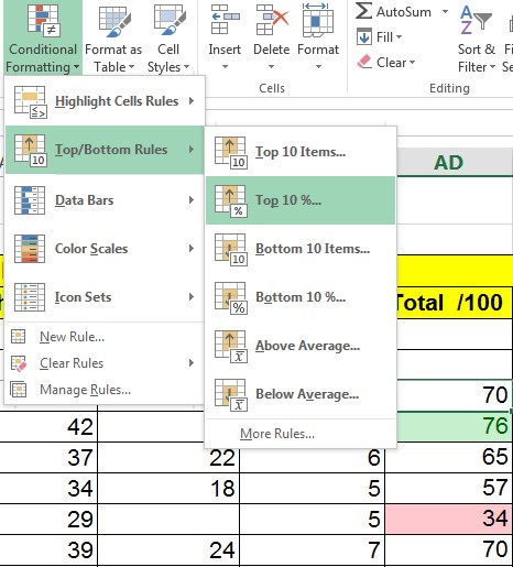
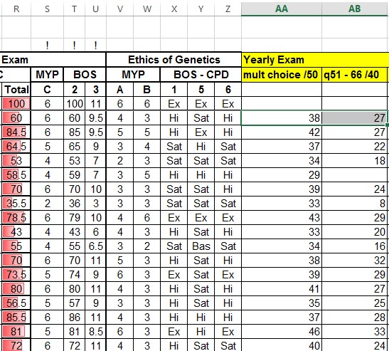
I also decided to add in ‘conditional formatting’ as an excellent way to graphically show results in a relative sense. This is shown in the image, below on the right, where bars graphically show the percentage grades of the students. This is a feature I have never used before but since finding out about it is one I will be using in future.
For the yearly results (column AD) I used conditional formatting to show the top 10% in green while the bottom 15% was filled in red. This is shown by the image to the left. Again a feature I have not used but will so in the future as a very convenient indicator of student performance at both ends of the spectrum. |
Also at the top of each sheet I have frozen the panes so when scrolling the titles, and what the marks are out of, can be seen continually. This can be seen in the image below where the top 6 rows are frozen and can be seen but I have scrolled down to the 107th row and beyond.
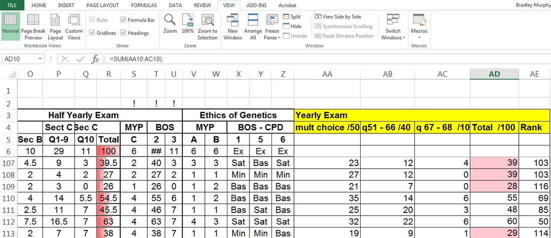

This is a feature of excel I have not used much of in the past but again it is very useful so will be using it in the future.
Using tabs in excel is very useful to logically categorise data as well as not avoiding too much data on one sheet. Formulae can link one sheet to another by including the name of the tab, an apostrophe, and then the reference of the field needed.
For example:
=raw!H7; used in the ‘sem 1 manipulated’ tab inserts data in this tab from the ‘raw’ tab.
This is shown in the image to the right which is part of the "Sem 1 manipulated tab"
The image below is of the raw data found in the 'raw' tab.
For many years I have used excel to determine averages, however during this course I learned how to get excel to round figures to the nearest whole figure. This is very useful for reports where you need to put in a grade as a whole number, eg ‘4’, rather than ‘4.43’
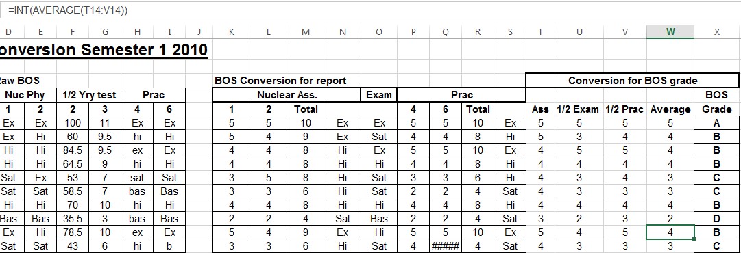
For example in the ‘sem 1 manipulated’ tab the formula ‘=INT(AVERAGE(T14:V14))’ includes the INT function which rounds a number down to the next lowest integer. This coupled with the average formula means the average grade is rounded to a whole number.
For example in the ‘sem 1 manipulated’ tab the formula ‘=INT(AVERAGE(T14:V14))’ includes the INT function which rounds a number down to the next lowest integer. This coupled with the average formula means the average grade is rounded to a whole number.
The above tab, along with others also have more ‘if’ statements.
In the ‘Sem2 reports’ tab I have the following formula:
=(raw!AA7+raw!AB7)/9*10
‘raw!’ takes the data from the ‘raw’ tab into the ‘Sem2 reports’ tab where data in ‘AA7’ and ‘AB7’ are added and then converted to a percentage (from being out of 90) by dividing by 9 and multiplying by 10. There are other ways of doing this, such as using a ‘percentage function or clicking the % button…
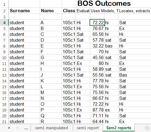
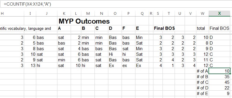
In the ‘Sem2 reports’ tab I also have the ‘countif’ formula to determine the number of grades A to E:
So from cells X4 to X124 if A is present it counted them of which there were 10; equivalent values were counted for the other grades as can be seen in the screenshot below.
So from cells X4 to X124 if A is present it counted them of which there were 10; equivalent values were counted for the other grades as can be seen in the screenshot below.